“A generating function is a clothesline on which we hang up a sequence of numbers for display” – Herbert Wilf, Generatingfunctionology

Counting bills

Consider the following problem:

You have an unlimited number of $1, $5, and $10 bills. How many ways are there to make $10?

Let’s work it out: we could use ten $1 bills; five $1 bills, and one $5 bill; two $5 bills; or a single $10 bill. That gives us four possible ways. While this works for small numbers, it quickly becomes tedious as the number of bills and denominations increases. Can we find a more systematic method, one that also generalizes to larger cases?

Let’s examine the problem again. Note that each denomination contributes some multiple of its value, so we can only possibly choose a set number of bills of each denomination. For $1 bills, we can take 0, 1, 2, or any other number up to 10. For $5 bills, we can take 0, 1, or 2. For $10 bills, we can only take 0 or 1.

So we have to find the number of valid combinations of these bills. Is there a way to encode these values so that they can be easily manipulated and the answer easily extracted? One seemingly random way to do this is to use polynomials. Let the exponent track the total sum and the coefficient track the number of ways to achieve that sum. So, for example, \(4 x^{12}\) would mean that there are 4 ways to add up our bills to get the value 12.

For the $1 bill, we construct the polynomial \(1 + x + \dots + x^{10}\) because we can achieve any sum by just choosing that number of $1 bills. For the $5 bill we have \(1 + x^5 + x^{10}\), and similarly for the $10 bills we have \(1 + x^{10}\). Note the presence of \(x^0\), this is because we can always choose zero of a given denomination.

Let’s multiply these three polynomials together and see what we get: \[(1 + x + \dots + x^{10}) \cdot (1 + x^5 + x^{10}) \cdot (1 + x^{10}) \\ = 1 + x + x^2 + x^3 + x^4 + 2x^5 + 2x^6 + 2x^7 + 2x^8 + 2x^9 + 4x^{10} + \cdots.\]

Notice that the coefficient next to \(x^{10}\) is 4. This is our desired answer! But that’s not all — now we also know how many ways the sums from 1 to 9 can be achieved!

It turns out the multiplication of polynomials models the way we choose bill combinations in this problem, and in general, it models the way we form subsets in similar combinatorial problems.

In this case, it doesn’t really save us much work, but the principle can help us crack many hard problems. Generating functions are one of those mathematical tools that must be used to be understood — they may feel a bit contrived, but they work extremely well in practice. This introductory problem is a good way to grasp the basics, but there is much more to generating functions!

Fibonacci numbers

One of the most famous integer sequences in mathematics is the Fibonacci sequence (A000045 in the OEIS). It gets its name from the Italian mathematician Leonardo of Pisa, known commonly as Fibonacci, who described them in his 1202 book Liber Abaci. Latin for “The Book of Calculation”, it also introduced, among other things, the Hindu–Arabic base 10 numerals to Europe. But this sequence has been known to humans for a lot longer than that, first appearing in the writings of Indian mathematicians around 200 BCE.

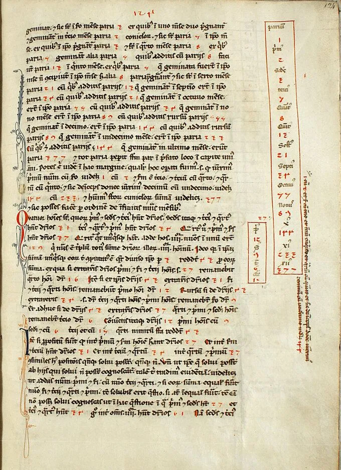A page from Liber Abaci containing the Fibonacci sequence in the right margin. Note the use of Arabic and Hindu numerals in red.

A given element in the Fibonacci sequence is defined as the sum of the two preceding elements, where the first two elements are given as 0 and 1. This can be expressed with the following recurrence relation \[F_0 = 0, \ F_1 = 1 \\ F_n = F_{n-1} + F_{n-2}, \quad n > 1.\]

Its first few members are: \[0, \; 1, \; 1, \; 2, \; 3, \; 5, \; 8, \; 13, \; 21, \; 34, \; 55, \; 89, \; 144, \; \dots\]

But what if we want to know, say, the 200th Fibonacci number? Would we have to solve the recurrence relation 200 times? It turns out that we don’t, because we can construct a closed-form formula for the \(n\)-th Fibonacci number! This can be done using generating functions!

This is because, essentially, a generating function is a way to represent an infinite sequence as the coefficients of a formal power series. The series being formal means that we are not concerned with its convergence, and the variable \(x\) is an indeterminate. So the infinite sequence \((a_0, a_1, a_2,…)\) can be expressed with the generating function \(\sum_{n=0}^{\infty} a_n x^n = a_0 + a_1 x + a_2 x^2 + \cdots\).

For example the sequence \((1, 1, 1, …)\) has \(\sum_{n=0}^{\infty} x^n = \frac{1}{1-x}\) as its generating function. Note that we can use the closed form of the series to represent the generating function.

Generating functions defined this way—as the coefficients of a geometric series—are called ordinary generating functions. There are many kinds of generating functions; I might mention some more in a future article. Each of them helps us solve a specific class of problems.

OK, back to the Fibonacci sequence. Let’s start by defining its generating function as \[F(x) = \sum_{n=0}^{\infty} F_n x^n.\]

Now recall the recurrence relation given above. We can use it to rewrite the series and get \[\begin{align*} F(x) &= F_0 + F_1 x + \sum_{n=2}^{\infty} F_n x^n \\ &= 0 + 1 x + \sum_{n=2}^{\infty} (F_{n-1} + F_{n-2}) x^n \\ &= x + x \sum_{n=2}^{\infty} F_{n-1} x^{n-1} + x^2 \sum_{n=2}^{\infty} F_{n-2} x^{n-2}. \end{align*}\]

We can now take care of the sums. Since \(F_0 = 0\) the first sum becomes \(0 + x \sum_{n=1}^{\infty} F_{n-1} x^{n-1}\). So by shifting indices both sums become \(\sum_{n=0}^{\infty} F_n x^n\). This is just our generating function! So substituting that in gives us the expression \[F(x) = x + x F(x) + x^2 F(x).\]

After factoring out \(F(x)\) we get \[F(x) = \frac{x}{1-x-x^2}.\]

At this point we could actually just take the Maclaurin series expansion of the above function to get each Fibonacci number. This is also interesting in itself but we want a closed form formula. So to continue we can use partial fraction decomposition to simplify the expression.

Let’s start by solving \( -x^2 - x + 1 = 0 \). We can plug the parameters into the quadratic equation to get the two roots \[\phi = \frac{1 + \sqrt{5}}{2}, \ \psi = \frac{1 - \sqrt{5}}{2}.\]

Now, continuing with the partial fraction decomposition, we get \[F(x) = \frac{x}{(1 - \phi x)(1 - \psi x)} = \frac{A}{1 - \phi x} + \frac{B}{1 - \psi x}.\]

After some fairly simple algebra we can conclude that \(A = \frac{1}{\sqrt{5}}\) and \(B = - \frac{1}{\sqrt{5}}\). Substituting that in, and noting that \(\sum_{n=0}^{\infty} (a x)^n = \frac{1}{1 - ax}\) we get the following expression \[\begin{align*} F(x) &= \frac{1}{\sqrt{5}} \left( \frac{1}{1 - \phi x} - \frac{1}{1 - \psi x} \right) \\ &= \frac{1}{\sqrt{5}} \left( \sum_{n=0}^{\infty} ( \phi x )^n - \sum_{n=0}^{\infty} ( \psi x )^n \right) \\ &= \sum_{n=0}^{\infty} \frac{\phi^n - \psi^n}{\sqrt{5}} x^n. \end{align*}\]

Since the coefficients of \(F(x)\) are the Fibonacci numbers \( F_n \) we now have the final closed form: \[F_n = \frac{\phi^n - \psi^n}{\sqrt{5}} = \frac{1}{\sqrt{5}} \left( \left( \frac{1 + \sqrt{5}}{2} \right)^n - \left( \frac{1 - \sqrt{5}}{2} \right)^n \right).\]

This expression is known as Binet’s formula, and generating functions aren’t the only way to derive it. But this procedure demonstrates how useful and surprisingly versatile they are.

Counting trees

Now let’s take a walk in the mathematical forest. This forest is made up of binary trees — a type of graph commonly used in computer science. They are rooted, and each tree node has at most 2 children.

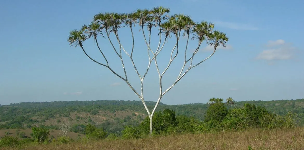Hyphaene compressa¹ would probably be in our forest. This specimen is a full binary tree with 31 nodes.

We may want to know how many ways there are to construct such a tree with \(n\) nodes. Like any combinatorial problem, the best way to solve it is to draw out the first few cases to see if we notice a pattern.

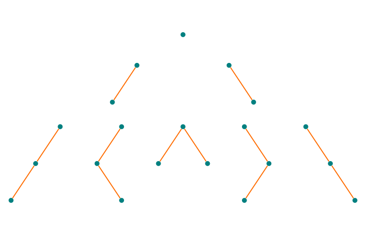All possible ways to construct binary trees with 1, 2, and 3 nodes.

Note that for 0 nodes, there is 1 way to construct an empty tree. Note also that we treat the right and left child as distinct.

After drawing out these trees for a while, you might notice that this problem becomes a bit recursive. The easiest way to construct new trees is to take the trees from the previous level and add new branches.

We can generalize this thinking if we consider only the root node of a tree with \(n\) nodes. It has a left subtree with \(0 \leq k \leq n-1\) nodes, and a right subtree with \(n-1-k\) nodes. We can then apply the rule of product and conclude that for a given \(k\) there are \(C_{k} \cdot C_{n-1-k}\) such trees.

Summing over all possible values of \(k\), we get the following recurrence relation \[C_n = \sum_{k=0}^{n-1} C_{k} C_{n-1-k}, \quad n \geq 1.\]

As stated above, our initial condition is \(C_0=1\). You can start plugging numbers in to verify that this lines up with the number of graphs we got earlier. This is nice and useful, but we want the coveted closed-form expression. This can be achieved using, you guessed it, generating functions!

Let’s define the generating function for Catalan numbers as \[C(x) = \sum_{n=0}^{\infty} C_n x^n.\]

Take the recurrence relation that we just derived and multiply both sides by \(x^n\). Now summing for \(n \geq 1\) yields \[\begin{align*} \sum_{n=1}^{\infty} \left(\sum_{k=0}^{n-1} C_k C_{n-1-k}\right) x^n &= \sum_{n=1}^{\infty} C_n x^n \\ &= \sum_{n=0}^{\infty} C_n x^n - C_0 \\ &= C(x) - 1. \end{align*}\]

Now, doesn’t the sum on the left look a bit familiar? It looks very similar to the formula for the discrete convolution of two infinite series, or the Cauchy product: \( \bigl( \sum_{i=0}^{\infty} a_{i} \bigr) \bigl( \sum_{j=0}^{\infty} b_{j} \bigr) = \sum_{k=0}^{\infty} \bigl( \sum_{l=0}^{k} a_{l} b_{k-l} \bigr)\). But for this to be an actual Cauchy product \(n\) would have to start from 0. We can fix this by letting \(m=n-1\) and factoring out \(x\), thus giving us \[\begin{align*} \sum_{n=1}^{\infty} \left(\sum_{k=0}^{n-1} C_k C_{n-1-k}\right) x^n &= x \sum_{n=1}^{\infty} \left(\sum_{k=0}^{n-1} C_k C_{n-1-k}\right) x^{n-1} \\ &= x \sum_{m=0}^{\infty} \left(\sum_{k=0}^{m} C_k C_{m-k}\right) x^m \\ &= x \left(\sum_{n=0}^{\infty} C_n x^n\right) \left(\sum_{n=0}^{\infty} C_n x^n\right) \\ &= x C(x)^2. \end{align*}\]

This demonstrates another powerful feature of generating functions: multiplication of generating functions yields the discrete convolution of their sequences. Another reason why they prove so useful in solving combinatorial problems, where convolutions show up regularly.

Continuing with the problem, we can now put the two sides together to get the expression \[C(x) - 1 = x C(x)^2.\]

This is a quadratic equation in \(C(x)\), so by the trusty quadratic formula we get \[C(x) = \frac{1 \pm \sqrt{1 - 4x}}{2x}.\]

Hmm we hit a fork in the road… What branch should we choose here?

Well, we know that \(C_0 = 1\) — that is just our initial condition. And we know that we can extract coefficients using the Maclaurin expansion \(C_n = \tfrac{C^{(n)}(0)}{n!}\). Thus it follows that \(C_0 = C(0)\).

So we just have to check which branch evaluates to 1 when \(x=0\). Our formula has division by zero, so we have to take the limit where \(x \to 0\). Doing this for both branches gives us \[\begin{align*} \lim_{x \to 0} \frac{1 + \sqrt{1 - 4x}}{2x} &= \frac{1+1}{0} = +\infty \\ \lim_{x \to 0} \frac{1 - \sqrt{1 - 4x}}{2x} &\overset{\mathrm{L’H}}{=} \lim_{x \to 0} \frac{2 (1 - 4x)^{-\frac{1}{2}}}{2} = 1. \end{align*}\]

Bingo — the minus branch is the correct one! Now we want to get a formula for the \(n\)-th coefficient of the power series expansion of this expression.

With the help of the old binomial series \(\sum_{n=0}^\infty \binom{\alpha}{n} x^n = (1 + x)^\alpha\), we can expand the radical to get \[(1-4x)^{\frac{1}{2}}= \sum_{k=0}^\infty \binom{\frac{1}{2}}{k}(-4x)^k.\]

The 0-th coefficient of this series is 1, so the numerator can be written as \[ 1- (1-4x)^{\frac{1}{2}}= -\sum_{k=1}^\infty \binom{\frac{1}{2}}{k}(-4x)^k. \]

Dividing this by \(2x\) and reindexing with \(n=k-1\) gives us the expansion \[\begin{align*} C(x) = \frac{1 - \sqrt{1 - 4x}}{2x} &= -\frac{1}{2} \sum_{k=1}^\infty \binom{\frac{1}{2}}{k}(-4)^k x^{k-1} \\ &= -\frac{1}{2} \sum_{n=1}^\infty \binom{\frac{1}{2}}{n+1}(-4)^{n+1} x^{n}. \end{align*}\]

So there we have it, the closed-form expression for our problem is \[C_n = -\frac{1}{2} \binom{\frac{1}{2}}{n+1}(-4)^{n+1}.\]

But yeah, this is way too ugly… Let’s try to simplify it a bit. The most obvious place to start is \(\binom{\frac{1}{2}}{n+1}\).

We usually define the binomial coefficients like \(\binom{a}{b} = \frac{a!}{b! (a-b)!}\). This won’t work in our case since \(a\) is not an integer, and thus \(a!\) is not defined.

To fix this let’s introduce the falling factorial \[a^{\underline{b}} = \prod_{k=0}^{b-1} (a - k) = a(a-1)\cdots(a - b + 1).\]

Now it clearly follows that \(a^{\underline{b}} = \frac{a!}{(a-b)!}\). Plugging this into the definition of the binomial coefficient, we get \(\binom{a}{b} = \frac{a^{\underline{b}}}{b!}\). Applying this to our coefficient, we have \[\binom{\frac{1}{2}}{n+1} = \frac{(\frac{1}{2})^{\underline{n+1}}}{(n+1)!} = \frac{\frac{1}{2} (\frac{1}{2} - 1) \cdots (\frac{1}{2} - (n+1 -1))}{(n+1)!}.\]

We can factor out \(\frac{1}{2}\) from each parenthetical and get \[\frac{\frac{1}{2} \frac{1}{2^n} (1 - 2) (1 - 4) \cdots (1 - 2n)}{(n+1)!} = \frac{(\frac{1}{2})^{n+1} \prod_{k=1}^n (1 - 2k)}{(n+1)!}.\]

Now, thinking ahead for a bit, we can factor out -1 from the product so that it cancels out the -4 in our original expression thus giving us \[\binom{\frac{1}{2}}{n+1} = \frac{(-1)^n \prod_{k=1}^n (2k - 1)}{2^{n+1} (n+1)!}.\]

We can now plug this expression into the full formula for \(C_n\). After some wrist exercise we get \[\begin{align*} C_n &= -\frac{1}{2} \; \frac{(-1)^n \prod_{k=1}^n (2k - 1)}{2^{n+1} (n+1)!} \; (-4)^{n+1} \\ &= \cancel{(-1)^{n+1}} \, \cancel{(-1)^{n+1}} \, \; \frac{4^{n+1}}{2^{n+2}} \; \frac{\prod_{k=1}^n (2k - 1)}{(n+1)!} \\ &= \frac{\cancel{2^{n+2}}}{\cancel{2^{n+2}}} \, \; 2^n \; \frac{\prod_{k=1}^n (2k - 1)}{(n+1)!} \\ &= 2^n \; \frac{\prod_{k=1}^n (2k - 1)}{(n+1)!}. \end{align*}\]

But we still have this cumbersome product in the numerator. Perhaps there is a way to write it in a closed form?

Consider the expression \[(2n)! = \prod_{k=1}^{2n} k = \left(\prod_{k=1}^{n} 2k\right)\left(\prod_{k=1}^{n} (2k-1)\right).\]

Now notice that we can factor 2 out of the even product to get \( \prod_{k=1}^{n} 2k = 2^n n!. \) Rearranging the full expression now gives us the identity \[\prod_{k=1}^n (2k-1) = \frac{(2n)!}{2^n n!}.\]

We’re in the final stretch now. We can plug this into our formula for \(C_n\). After canceling out \(2^n\) we finally get \[C_n = \frac{(2n)!}{n! (n+1)!} = \frac{1}{n+1} \binom{2n}{n}.\]

Phew, so there we are. A nice closed-form expression for our tree-counting problem. Well, not just the tree-counting problem… This expression generates the sequence: \[1, \; 1, \; 2, \; 5, \; 14, \; 42, \; 132, \; 429, \; 1430, \; 4862, \; 16796, \; \dots\]

This sequence (A000108 in the OEIS) is quite special; its members are called the Catalan numbers. They get their name after Eugène Charles Catalan, a 19th-century Belgian mathematician, but they were described much earlier by the Mongolian mathematician Minggatu in the 1730s and Leonhard Euler in 1751.

What makes this sequence so special is the fact that it shows up so frequently. For the sake of brevity, I will just list out the most famous occurrences here:

• The number of correct ways to arrange \(n\) pairs of parenthesis. This is directly equivalent to the number of possible Dyck words of length \(2n\).
• The number of ways to triangulate a convex \((n+2)\)-gon. This is the way Euler discovered Catalan numbers.
• The number of ways to construct a full binary tree with \(n+1\) labeled leaves.
• The number of noncrossing partitions of the set of \(n\) elements.
• The number of ways to form a “mountain range” with n up-strokes and n down-strokes that all stay above the original line.
• The number of paths on a \(n \times n \) square grid from bottom to top that do not cross the main diagonal.

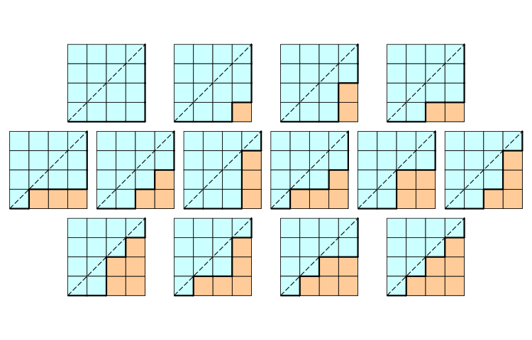All possible ways to construct these paths on a \(4 \times 4\) grid. If we count them, we get 14 — the 4th Catalan number!

There are many, many more. Wikipedia lists a couple more, and Richard P. Stanley’s definitive monograph Catalan Numbers has some 200 pages worth of dense information on just this one sequence. Stanley also produced some slides that summarize this topic and elucidate some of the examples given above.

Conclusion

This is only the tip of the generating function iceberg. They are a really useful mathematical tool that is also fun to work with. I’ll probably write another article about them.

Catalan numbers are also a fascinating topic on their own. I believe that the OEIS entry about them is the longest one on the entire site! They really are that special.

Literature

For generating functions, there really is no book better than excellently named generatingfunctionology by Herbert Wilf. For Catalan numbers, I have already mentioned Stanley’s Catalan Numbers.

As always, 3Blue1Brown has an excellent video on generating functions. SackVideo also has a good video on the topic, focusing more on the problem of counting binary trees.

~ Well, that’s it for this entry! Have fun and happy hacking!